[PRML] Ch 1.2 Probability Theory

This post is summary of the book Pattern Recognition and Machine Learning by Christopher M. Bishop

A lot of explanations in this page has been quoted from the book directly because most of the content is about definitions used in probability theory

1.2 Probability Theory

• Uncertainty is a key concept in the field of pattern recognition
• uncertainty arises through:
  • noise on measurements
  • finite size of data sets
• Probability Theory provides:
  • a consistent framework for quantification and manipulation of uncertainty
  • forms one of the central foundations for pattern recognition
• when probability theory is combined with Decision Theory:
  • allows us to make optimal predictions given all the information available to us
  • the information provided may be incomplete or ambiguous
  • will be discussed in Section 1.5

Example: apple and oranges

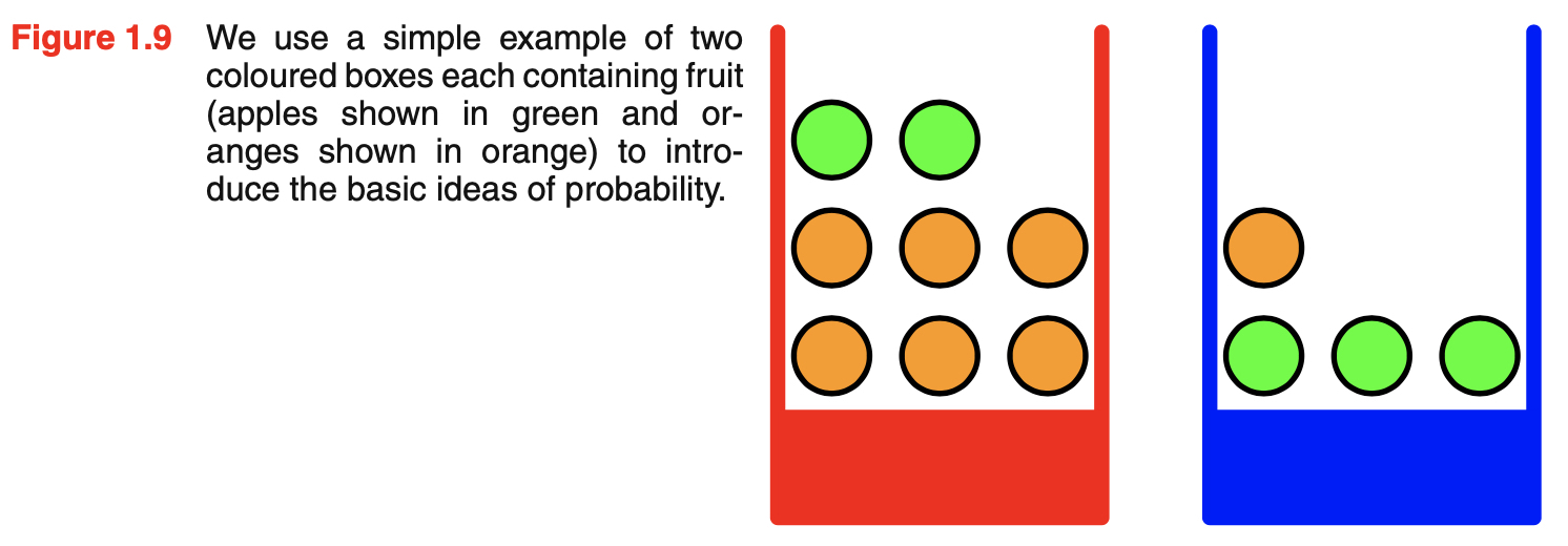
• two boxes of fruits from which an item of fruit is randomly selected and replaced
• suppose this process is repeated many times
  • equally likely to select any of the pieces of fruit in the box
• red box:
  • 2 apples and 6 oranges
  • 40% of the time pick red box
• blue box:
  • 3 apples and 1 orange
  • 60% of the time pick blue box

• random variables:
  • identity of the box:
    • denoted by B
    • possible values:
      • r: red box
      • b: blue box
  • identity of the fruit
    • denoted by F
    • possible values:
      • a: apple
      • o: orange
• probabilities of incidents:
  • probability of selecting the red box
    • $P(B = r) = \frac{4}{10}$
  • probability of selectinb the blue box
    • $P(B = b) = \frac{6}{10}$
• probabilities must lie in the interval [0,1] by definition
• the sum of probabilities of mutually exclusive events that include all possible outcomes must be one
  • in this example, the chosen box must be either red or blue
  • $P(B) = P(B = r) + P(B = b) = 1$

The Rules of Probability

• two elementary rules of probability are sum rule and product rule
• in order to derive these rules of probability, we will consider more general example involving two random variables $X$ and $Y$
  • X can take any values $x_i, i = 1, …, M$
  • Y can taky any values $y_j, j = 1, …, L$
  • a total of $N$ trials in which we sample both of the variables $X$ and $Y$
  • $n_{ij}$: number of trials which $X = x_i$ and $Y = y_j$
  • $c_i$: number of trials which $X$ takes the value $x_i$ regardless of the value of $Y$
  • $r_j$: number of trials which $Y$ takes the value $y_j$ regardless of the value of $X$

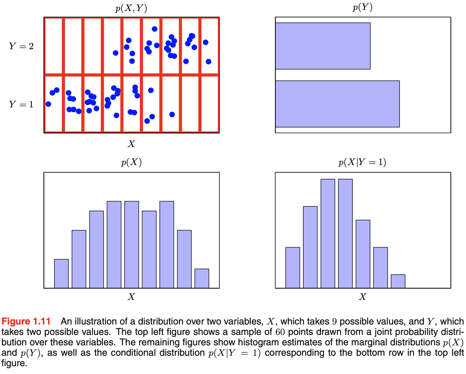
• $p(X = x_i, Y = y_j)$: probability that $X = x_i$ and $Y = y_j$
  • this is called the joint probability of $X = x_i$ and $Y = y_j$
  • the number of points falling in the cell $i,j$ as a fraction of the total number of points

\[p(X=x_i, Y=y_j) = \frac{n_{ij}}{N} \tag{1.5}\]

• here, we are implicitly considering the limit $N \rightarrow \infty$
  • this is the Frequentist view of probability
  • Bayesian perspective about probability will also be introduced later
• $p(X=x_i)$: probability that $X$ takes the value $x_i$ irrespective of the value of Y
  • this is called the marginal probability
  • the fraction of the total number of points that fall in column $i$

\[p(X=x_i)= \frac{c_i}{N} \tag{1.6}\]

• number of instances in column $i$ in Figure 1.10 is just the sum of the number of instances in each cell of that column
  • $c_i = \sum_j n_{ij}$
  • therefore following equation can be derived from (1.5) and (1.6)

\[p(X=x_i)= \sum_{j=1}^L p(X=x_i, Y=y_j) \tag{1.7}\]

• this is the sum rule of probability

• $p(Y=y_j \vert X=x_i)$: probability of $P(Y=y_j)$ when the value of $X$ is given as $X=x_i$

  • this is called the conditional probability of $Y = y_j$ given $X=x_i$
  • the fraction of the point in column $i$ that fall in cell $i,j$

\[p(Y=y_j \vert X= x_i) = \frac{n_{ij}}{c_i} \tag{1.8}\]

• from (1.5), (1.6), and (1.8), we can derive the following relationship

\[p(X=x_i, Y=y_j) = \frac{n_{ij}}{N} = \frac{n_{ij}}{c_i} \cdot \frac{c_i}{N} = p(Y = y_j \vert X=x_i)p(X=x_i) \tag{1.9}\]

• this is the product rule of probability

• the rules of probability

  • sum rule \(p(X) = \sum_{Y} p(X,Y) \tag{1.10}\)
  • product rule \(p(X,Y) = p(Y|X)p(X) \tag{1.11}\)

Bayes’ Theorem

• from the symmetry property of product rule, we can obtain Bayes’ theorem
  • symmetry property of product rule
  \[p(X,Y) = p(Y|X)p(X) = p(X|Y)p(Y) = p(Y,X)\]
  • Bayes’ Themorm
  \[p(Y|X) = \frac{p(X|Y)p(Y)}{p(X)} \tag{1.12}\]
• Bayes’ theorem plays a central role in pattern recognition and machine learning
• Bayes’ theorem can be expressed in terms of quantities appearing in the numerator using the sum rule
  • denominator can be seen as the normalization constant
    • because the sum of conditional probability must add up to one

\[p(X) = \sum_Y p(X|Y)p(Y) \tag{1.13}\] \[p(Y|X) = \frac{p(X|Y)p(Y)}{\sum_Y p(X|Y)p(Y)}\]

• figure below visualizes joint, marginal, and conditional distributions
  • visualization is important part of statisical pattern recognition and will be explored later

Summary with numbers

• going back the the apples and oranges example
  • short recap: \(p(B=r) = \frac{4}{10} \tag{1.14}\) \(p(B=b) = \frac{6}{10} \tag{1.15}\)
• conditional probabilities:
  • the probability of picking apples in the blue box: \(p(F=a|B=r)= \frac{1}{4} \tag{1.16}\)
  • the probability of picking oranges in the blue box: \(p(F=o|B=r)= \frac{3}{4} \tag{1.17}\)
  • the probability of picking apples in the red box: \(p(F=a|B=b) = \frac{3}{4} \tag{1.18}\)
  • the probability of picking oranges in the blue box: \(p(F=o|B=b) = \frac{1}{$} \tag{1.19}\)

• note that all possibile events of the given condition must sum up to one \(p(F=a|B=r) + p(F=o|B=r) = 1 \tag{1.20}\) \(p(F=a|B=b) + p(F=o|B=b) = 1 \tag{1.21}\)

• sum and product rules of probability to evaluate the overall probability of choosing an apple

\[\begin{align*} p(F=a) &= p(F=a|B=r)p(B=r) + p(F=a|B=b)p(B=b) \\ &= \frac{1}{4} \times \frac{4}{10} + \frac{3}{4} \times \frac{6}{10} = \frac{11}{20} \tag{1.22} \end{align*}\]

• using the sum rule, $p(F=o) = 1-\frac{11}{20} = \frac{9}{20}$

• suppose we are told which fruit has been selected, and it’s orange, and want to find out which box it came from

  • we don’t know $p(B=r \vert F=o)$ from the information given
  • but we know $p(F=o \vert B=r)$, $p(B=r)$, and $p(F=o)$
  • therefore, we can use Bayes’ theorem to find out the answer for $p(B=r \vert F=o)$

\[\begin{align*} p(B=r|F=o) &= \frac{p(F=o|B=r)p(B=r)}{p(F=o)} \\ &= \frac{3}{4} \times \frac{4}{10} \times \frac{20}{9} = \frac{2}{3} \tag{1.23} \end{align*}\]

• using the Bayes’ theorem, we could make predictions about which box the fruit came from
  • before we were told which fruit has been selected, the most complete information we had about box was $p(B)$
    • this is called prior probability because it is the probability available before we obtained the data
  • after we observed the identity of the fruit, we could update our prior probability with the given data and got $p(B \vert F)$
    • this is called posterior probability because it in the probability obtained after we have observed F
• for this example, the probability of selecting the red box has significantly increased after we observed that the selected fruit is an orange
  • this is becuase there were more oranges in the red box than in the blue box
  • this concept is very important later since it allows us to update our prediction after we observe data
    • nobody wants to make poor guesses forever!
• two variables X and Y are said to be independent if $p(X,Y) = p(X)p(Y)$
  • we can prove this from the product rule
  • if $p(X,Y) = p(X)p(Y)$, $p(Y \vert X) = p(Y)$
  • this means conditional probability of Y given X is independent of the value of X

1.2.1 Probability densities

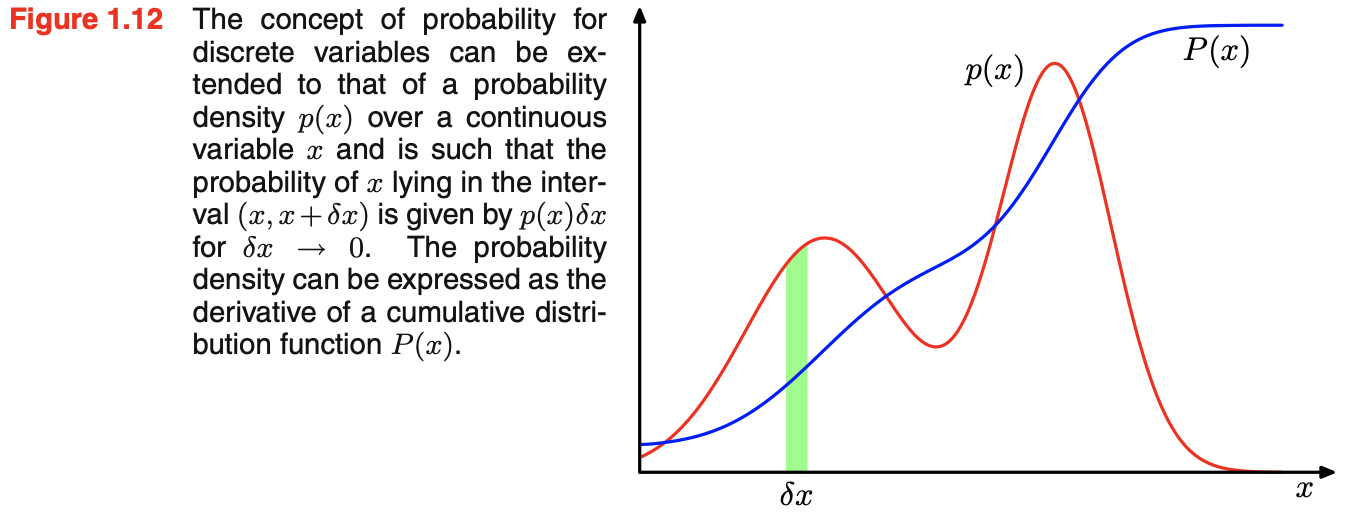
• if the probability of a real-valued variable $x$ falling in the interval $(x, x+ \delta x)$ is given by $p(x)\delta x$ for $\delta x \rightarrow 0$, then $p(x)$ is called the probability density over $x$
• the probability that $x$ will lie in an interval $(a, b)$ is given by the following equation \(p(x \in (a,b)) = \int_a^b p(x)dx \tag{1.24}\)
• probabilities are nonnegative by definition
• the value of $x$ must lie somewhere on the real axis
• therefore, the probability density $p(x)$ must satisfy the two conditions

\[p(x) \geq 0 \tag{1.25}\]

$\int_{-\infty}^{\infty} p(x) dx = 1 \tag{1.26}$

Change of Variables

• nonlinear change of variables must be processed with special care due to Jacobian factor
  • consider a change of variable $x = g(y)$
  • then a function $f(x)$ becomes $\tilde{f}(y) = f(g(y))$
  • this works the same in probability density
  • consider a probability density $p_x(x)$ that corresponds to a density $p_y(y)$ with respect to the new variable y
  • observations falling in the range $(x, x + \delta x)$ will, for small values of $\delta x$, be transformed into the range $(y, y+\delta y)$ where $p_x(x)\delta x \simeq p_y(y)\delta y$
  \[p_y(y) = p_x(x) \left\vert \frac{dx}{dy} \right\vert = p_x(g(y))\vert(g'(y))\vert \tag{1.27}\]
• the concept of the maximum of a probability density is dependent on the choice of variable

---

• the probability that $x$ lies in the interval $(-\infty, z)$ is given by the cumulative distribution function
  • satisfy $P’(x) = p(x)$ as shown in Figure 1.12

\(P(z) = \int_{-\infty}^{z} p(x)dx \tag{1.28}\)

• if we have several continuous variable $x_1, …, x_D$, denoted collectively by the vector $\mathbf x$, then we can define a joint probability density $p(x) = p(x_1, …, x_D)$
• the probability of $\mathbf x$ falling in an infinitesimal volume $\delta \mathbf x$ containing the point $\mathbf x$ is given by $p(\mathbf x)\delta \mathbf x$

\[p(\mathbf x) \geq 0 \tag{1.29}\]

\(\int p(\mathbf x)d(\mathbf x) = 1 \tag{1.30}\)

• if $x$ is discrete variable, then $p(x)$ is called a probability mass function
  • because it can be regarded as a set of ‘probability masses’ concentrated at the allowed values of $x$
• sum and product rules of probability and Bayes’ theorem apply equally to the case of probability densities or to combinations of discrete and continuous variables

\[p(x) = \int p(x,y)dy \tag{1.31}\] \[p(x,y) = p(y\vert x)p(x) \tag{1.32}\]

1.2.2 Expectations and covariances

• the average value of some function $f(x)$ under a probability distribution $p(x)$ is called the expectation of f(x)
  • denoted by $\mathrm E[f]$
  • one of the most important operations involving probabilities
  • the average is weighted by the relative probabilities of the different values of $x$
• for discrete distribution, expectation is given by

\[\mathrm E[f] = \sum_xp(x)f(x) \tag{1.33}\]

• for continuous variables, expevtations are expressed in terms of an integration with respect to the corresponding probability density

\[\mathrm E[f] = \int p(x)f(x)dx \tag{1.34}\]

• if we are given a finite number N of points drawn from the probability distribution or probability density, then the expectation can be approximated as a finite sum over these points
  • the approximation becomes exact in the limit $N \rightarrow \infty$

\[\mathrm E[f] \simeq \frac{1}{N} \sum_{n=1}^Nf(x_n) \tag{1.35}\]

• for the case of multiple variables, we can use a subscript to indicate which variable is being averaged over

\[\mathrm E_x[f(x,y)] \tag{1.37}\]

• this denotes the average of the function $f(x,y)$ with respect to the distribution of $x$
  • $E_x[f(x,y)]$ will be a function of y
• conditional expectation with respect to a conditional distribution is analogus with the definition for continuous variables

\[\mathrm E[f\vert y] = \sum_x p(x \vert y)f(x) \tag{1.37}\]

• the variance of $f(x)$ provides a measure of how much variability there is in $f(x)$ around its mean value $\mathrm E[f(x)]$

\[var[f] = \mathrm E[(f(x)-\mathrm E[f(x)])^2] \tag{1.38}\]

• variance can be written in terms of the expectations of $f(x)$ and $f(x)^2$

\[var[f] = \mathrm E[f(x)^2] - \mathrm E[f(x)]^2 \tag{1.39}\]

• we can consider the variance of the variable $x$ itself

\[var[x] = \mathrm E[x^2] - \mathrm E [x]^2 \tag{1.40}\]

• for two random variables x and y, the covariance expresses the extent to which $x$ and $y$ vary together
  • if x and y are independent, then their covariance vanishes

\[cov[x,y] = \mathrm E_{x,y}[\{x - \mathrm E[x]\}\{y - \mathrm E [y]\}] = \mathrm E_{x,y}[xy] - E[x]E[y] \tag{1.41}\]

• in the case of two vectors of random variable $x$ and $y$, the covariance is a matrix
  • $cov[x] \equiv cov[x,x]$

\[cov[x,y] = \mathrm E_{x,y}[\{ \mathbf x - \mathrm E[ \mathbf x]\}\{ \mathbf y^T - \mathrm E[\mathbf y^T]\}] = \mathrm E_{x,y}[\mathbf x \mathbf y^T] - \mathrm E[\mathbf x] \mathrm E[\mathbf y^T] \tag{1.42}\]