[PRML] Ch 1.1 Example: Polynomial Curve Fitting

This post is summary of the book Pattern Recognition and Machine Learning by Christopher M. Bishop

1.1 Example: Polynomial Curve Fitting

• in this part of the chapter we will try to solve a simple regression problem
  • training set: N observations of x with corresponding target values t
    • \({\mathbf x} \equiv (x_1, ..., x_N)^T\), \({\mathbf t} \equiv (t_1, ..., t_N)^T\)
  • target values are generated from the function \(\sin(2 \pi x)\) with some random noise
    • $t_i = \sin(2 \pi x_i) + \epsilon_i$
    • this random noise allows us to possess an underlying regularity
    • this noise might arise from:
      • intrinsically stochastic process
      • more typically from unobserved sources of variability
    • however, individual observations are corrupted by this random noise
  • the figure below shows the data

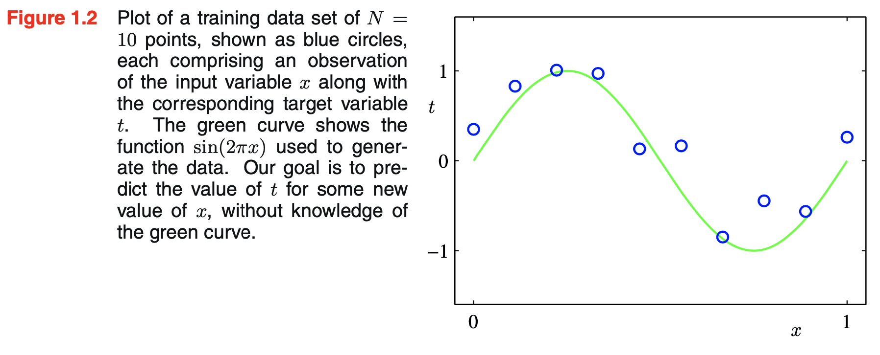
Our Goal is to successfully predict $\hat{t}$ for new input value $\hat{x}$ by exploiting the given training data

• Generalization is the key to successful representation of the target values because:
  • the given data set is finite
  • the given data set is corrupted with random noise
• Other theories will be introduced later in this book but for now, we will consider a simple approach based on curve fitting
  • Probability theory provides framework for expressing uncertainty in a precise and quantitative manner (Section 1.2)
  • Decision theory allows us ot exploit probabilistic representation in order to make predictions that are optimal according to appropriate criteria (Section 1.5)
• we shall fit the data using a polynomial function of the following form

\[y (x, w) = w_0 + w_1x + w_2x^2 + ... + w_Mx^M = \sum_{j=0}^Mw_jx^j \tag{1.1}\]

• although the polynomial funciton \(y(x, w)\) is a nonlinear function of x, it is a linear function of the coefficients w
  • this means if we consider x to be unknown parameter and w is it’s known coefficient, y is a nonlinear function of x because terms like $x^2, x^3, …, x^M$ exists
  • however, if we consider w as the unknown parameter, then y is a linear combination of $w_0, w_1, …, w_M$
  • these kind of functions are called linear models and will be discussed later

Error Function

• to achieve our goal, we have to find coefficients w using given training data
• in addition, we need a metric or standard to evaluate if our model is doing a good job or not
• one way to measure this is by using the error function
  • error function measures the misfit between the function $y(x, w)$ and the training set data points
  • our aim is to find the values of coefficients that can minimize this error function
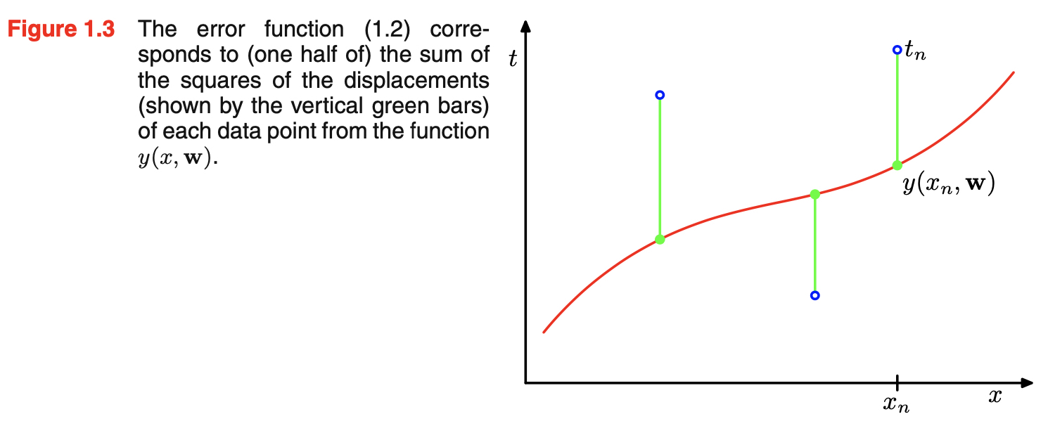
  • sum of squares of the errors are widely used

\[E(x) = \frac{1}{2}\sum_{n=1}^N\{y(x_n,w)-t_n\}^2 \tag{1.2}\]

• the factor of 1/2 is included for later convenience
  • it makes computation easier when you take the derivative of the error function
• because this function is nonnegative, it’s minimum value is zero and it’s value is zero if, and only if \(y(x_i,w) = t_i\) for $i = 1, …, N$
• geometric interpretation of the sum-of-squares error function is shown below

• because the error function is a quadratic function of the coefficients w, its derivatives with respect to the coeffcients will be linear in the elements of w
  • quadratic function means that the all terms in the functional expression f(w_1, w_2, …, w_n) have order two
• since $1, x, x^2, …, x^M$ are all linearly independent, there exists a unique solution which minimizes the error function
  • it is linearly independent because all the sample are assumed to be independent and identically distributed (i.i.d)
• this unique solution will be denoted $w^*$ and the resulting polynomial is given by the function $y(x, w^*)$

Model Selection

• choosing M of the polynomial remains a problem
  • this will turn out to be example of an important concept called model comparison or model selection

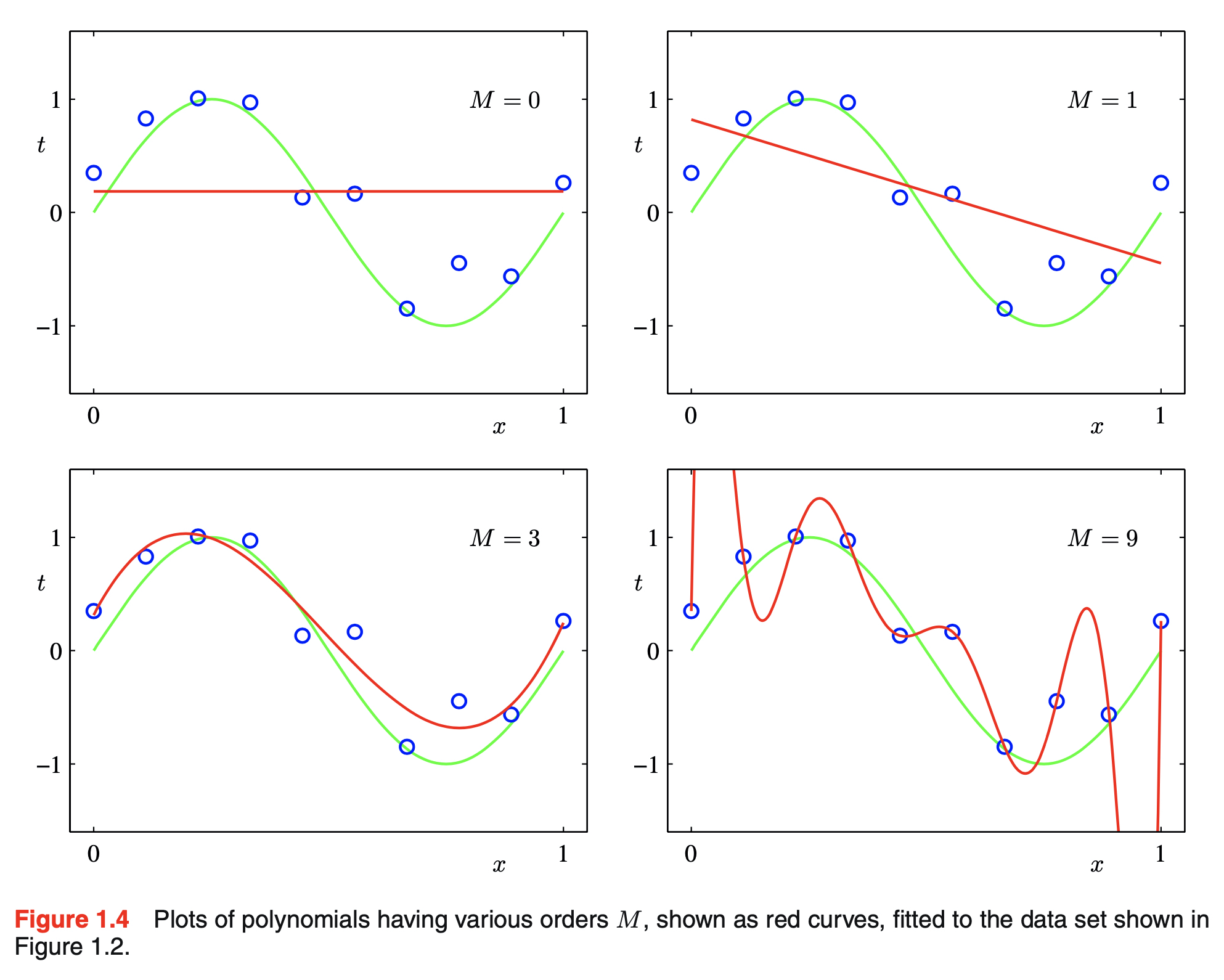
• as shown in the figure, if M is too small, the function gives poor representation of the real function $\sin(2 \pi x)$
  • this is called under-fitting
• on the other hand, if M is too big, the polynomial passes exactly through each data point but shows great oscillation between the data points
  • this is called over-fitting
• reminder, our goal is to achieve good-generalization by making accurate predictions for new data
• to accomplish this, we can separate the data into train and test set and measure the performance for each M
  • the measurement can be done by evaluating the residual value of $E(w^*)$ for training and test set separately
  • test set must not be used when finding $w^*$

  • it is more convenient to use root-mean-square in this case

    \[E_{RMS} = \sqrt{2E(W^*)/N} \tag{1.3}\]
    • N accounts for the difference in data sizes
    • square root ensures that $E_{RMS}$ is measured on the same scale as the target variable t
  • test set gives us clues about how well the polynomial will predict the values of t for new data observations of x
• with small values of M, the test and the training erors are both high as shown below

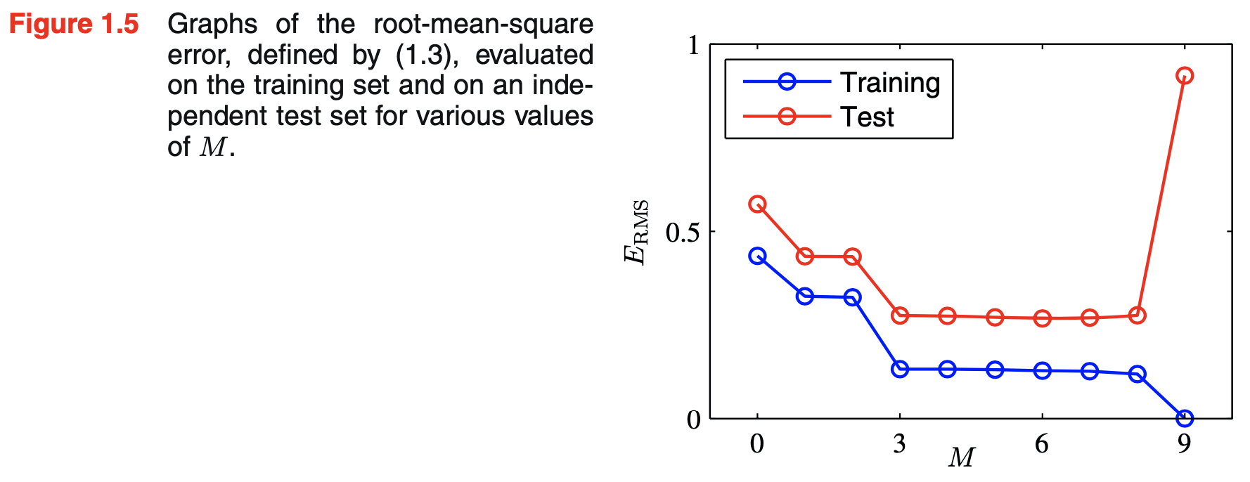
• if M gets too high, training error might drop but test error increases dramatically
  • this is the result of failure of generalization
  • also called over-fitting
• it seems that suitable choice of M is $3 \leq M \leq 8$
• it might seem odd that inreasing M from 3 to 9 makes things worse
  • however, it is shown that as we increase M, the magnitude of the coefficients gets larger dramatically
  • the polynomial might get the given data points correct but oscillates greatly between the data points
    • unable to interpolate between the data points
  • because our data conatains random noise, it can be said that with large values of M, the polynomials are becoming increasingly tuned to the random noise on the target values
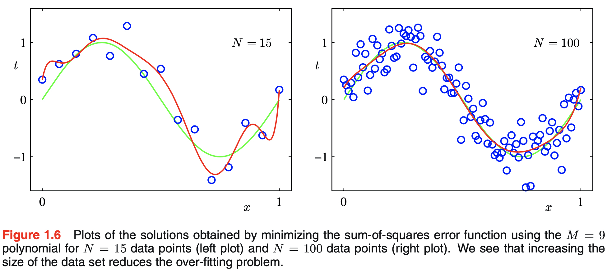
• over-fitting becomes less of a problem with bigger datasets with given model complexity as shown in the figure below
  • note that number of parameters is not necessarily the most appropriate measure of model complexity
    • this will be discussed in Chapter 3

• over-fitting problem can be understood in following approaches:
  • Maximum likelihood: over-fitting can be understood as a general property of maximum likelihood
    • least squares approach is a specific case of maximum likelihood
    • will be dicussed in Section 1.2.5
  • Bayesian approach: by adopting bayesian approach, over-fitting problem can be avoided
    • effective number of parameters adapts automatically to the size of the data set
      • doesn’t matter if the number of parameters greatly exceed the number of data points
    • will be discussed later

Regularization

• regularization involves adding penalty term to the error function (1.2) in order to discourage the coefficients from reaching large values
  • this caused problem as M increased in the previous section

\[\tilde{E}(x) = \frac{1}{2} \sum_{n=1}^{N} \{y(x_n, w) - t_n\}^2 + \frac{\lambda}{2}\|w\|^2 \tag{1.4}\]

• $|w|$ and the coefficient $\lambda$ emposes regulation to the error term
  • if these terms increase, the function $y(x, w)$ will have to do a better job in predicting the target value to keep the error low
  • it governs the relative importance of the regularization term compared with the sum-of-squares error term
• coefficient $w_0$ is omitted from the regularizer because its inclusion causes the results to depend on the choice of origin for the target variable
  • it may be included with its own regularization coefficient
• the error function in (1.4) can be minimized exactly in closed form
  • simply put, regularization term doesn’t change the fact that the error function has unique solution
• the particular case of a quadratic regularizer is called ridge regression
  • in the context of neural networks, this approach is known as weight decay

The impact of regularization term $\lambda$

• the result of the polynomial differs depending on the value of %\lambda% while the value of M stays constant
  • when $\lambda = -18$, the over-fitting problem has been alleviated

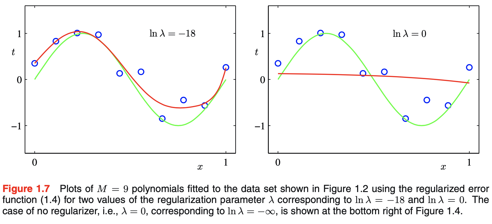
• too much suppression with large value of $\lambda$ results in poor fit
  • the effects of $\lambda$ is shown in the figure below

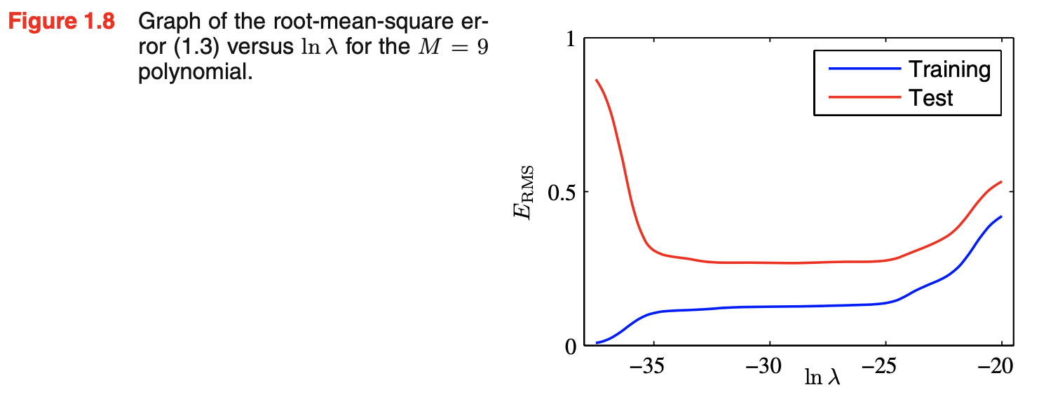
• $\lambda$ controls the effective complexity of the model and hence determines the degree of over-fitting
  • suitable value for the model complexity has to be determined in order to use this approach of minimizing an erorr function